|
AP Statistics - Chapter 3 Test DO NOT WRITE ON THIS TEST SHEETPart I – Multiple Choice: Circle the letter of the best answer on your answer sheet |
|
1. |
A study is conducted to determine if one can predict the yield of a crop based on the amount of yearly rainfall. The response variable in this study is |
|
|
A) |
yield of the crop. |
|
B) |
amount of yearly rainfall. |
|
C) |
the experimenter. |
|
D) |
either bushels or inches of water. |
|
|
A researcher measures the height (in feet) and volume of usable lumber (in cubic feet) of 32 cherry trees.
The goal is to determine if volume of usable lumber can be estimated from the height of a tree. The results are plotted below.
|
2. |
The scatterplot above suggests that |
|
|
A) |
there is a positive association between height and volume. |
|
B) |
there is an outlier in the plot. |
|
C) |
both a and b. |
|
D) |
neither a nor b. |
|
3. |
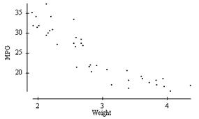
The graph below plots the gas mileage (miles per gallon, or MPG) of various 1978 model cars versus the weight of these cars in thousands of pounds.
In the graph, the points denoted by the plotting
symbol x correspond to cars made in |
|
|
A) |
in 1978 there was little difference between Japanese cars and cars made in other countries. |
|
B) |
in 1978 Japanese cars tended to be lighter in weight than other cars. |
|
C) |
in 1978 Japanese cars tended to get poorer gas mileage than other cars. |
|
D) |
the plot is invalid. A scatterplot is used to represent quantitative variables, and the country that makes a car is a qualitative variable. |

|
4. |
Consider the scatterplot below.
According to the scatterplot, which of the following is a plausible value for the correlation coefficient between weight and MPG? |
|
|
A) |
+0.2. |
|
B) |
–0.9. |
|
C) |
+0.7. |
|
D) |
–1.0. |
|
5. |
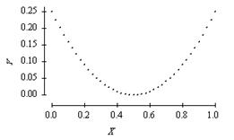
Consider the scatterplot below of two variables X and Y.
We may conclude that |
|
|
A) |
the correlation between X and Y must be close to 1 since there is a nearly perfect relation between them. |
|
B) |
the correlation between X and Y must be close to –1 since there is a nearly perfect relation between them, but it is not a straight-line relation. |
|
C) |
the correlation between X and Y is close to 0. |
|
D) |
the correlation between X and Y could be any number between –1 and +1. Without knowing the actual values of X and Y we can say nothing more. |
|
6. |
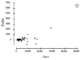
The profits (in multiples of $100,000) versus the sales (in multiples of $100,000) for a number of companies are plotted below. The correlation between profits and sales is 0.814. Suppose we removed the point that is circled from the data represented in the plot. The correlation between profits and sales would then be
|
|
|
A) |
0.814. |
|
B) |
larger than 0.814. |
|
C) |
smaller than 0.814. |
|
D) |
either larger or smaller than 0.814; it is impossible to say which. |
|
7. |
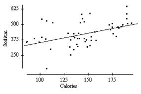
Below is a scatterplot of the calories and sodium content of several brands of meat hot dogs. The least-squares regression line has been drawn in on the plot.
Based on the least-squares regression line in this scatterplot, one would predict that a hot dog containing 100 calories would have a sodium content of about |
|
|
A) |
70. |
|
B) |
350. |
|
C) |
400. |
|
D) |
600. |
|
8. |
The fraction of the variation in the values of y that is explained by the least-squares regression of y on x is |
|
|
A) |
the correlation coefficient. |
|
B) |
the slope of the least-squares regression line. |
|
C) |
the square of the correlation coefficient. |
|
D) |
the intercept of the least-squares regression line. |
|
9. |
In a statistics course a linear regression equation was computed to predict the final exam score from the score on the first test. The equation of the least-squares regression line was
where y represents the final exam score and x is the score on the first exam. Suppose Joe scores a 90 on the first exam. What would be the predicted value of his score on the final exam? |
|||
|
A) |
91. |
||
|
B) |
89. |
||
|
C) |
81. |
||
|
D) |
It cannot be determined from the information given. We also need to know the correlation. |
||
|
10. |
The least-squares regression line is |
|
|
A) |
the line that makes the square of the correlation in the data as large as possible. |
|
B) |
the line that makes the sum of the squares of the vertical distances of the data points from the line as small as possible. |
|
C) |
the line that best splits the data in half, with half of the points above the line and half below the line. |
|
D) |
all of the above. |
|
11. |
Which of the following is true of the least-squares regression line? |
|
|
A) |
The slope is the change in the response variable that would be predicted by a unit change in the explanatory variable. |
|
B) |
It always passes through the point (J , M), the means of the explanatory and response variables, respectively. |
|
C) |
It will only pass through all the data points if r = ± 1. |
|
D) |
All of the above. |
|
12. |
A researcher wishes to study how the average weight Y (in kilograms) of children changes during the first year of life. He plots these averages versus the age X (in months) and decides to fit a least-squares regression line to the data with X as the explanatory variable and Y as the response variable. He computes the following quantities. r = correlation between X and Y = 0.9 J = mean of the values of X = 6.5 M = mean of the values of Y = 6.6 sJ = standard deviation of the values of X = 3.6 sM = standard deviation of the values of Y = 1.2 The slope of the least-squares line is |
|
|
A) |
0.30. |
|
B) |
0.88. |
|
C) |
1.01. |
|
D) |
3.0. |
|
13. |
In a study of 1991 model cars, a researcher found that the fraction of the variation in the price of cars that was explained by the least-squares regression on horsepower was about 0.64. For the cars in this study, the correlation between the price of the car and its horsepower was found to be positive. The actual value of the correlation |
|
|
A) |
is 0.80. |
|
B) |
is 0.64. |
|
C) |
is 0.41. |
|
D) |
cannot be determined from the information given. |
|
14. |
A scatterplot of the calories and sodium content of several brands of meat hot dogs is shown below. The least-squares regression line has been drawn in on the plot. Referring to this scatterplot, the value of the residual for the point labeled x
|
|
|
A) |
is about 40. |
|
B) |
is about 1300. |
|
C) |
is about 425. |
|
D) |
cannot be determined from the information given. |
|
15. |
The least-squares regression line is fit to a set of data. If one of the data points has a positive residual, then |
|
|
A) |
the correlation between the values of the response and explanatory variables must be positive. |
|
B) |
the point must lie above the least-squares regression line. |
|
C) |
the point must lie near the right edge of the scatterplot. |
|
D) |
all of the above. |
Part II – Free Response: Show all work on the answer sheet. Write clearly and completely.
1. It has been theorized that workers are less likely to quit their jobs when wages are high than when they are low. In 1986, the paper “Investigating the Causal Relationship Between Quits and Wages” compared average hourly wage (x) to quit rate (y), which was expressed as a percentage of employees who quit that year, for 15 different industries. The regression results are as follows:
quit rate = 4.86 – .35wages, r = -.854 and r2 = .729
a) Find the estimated quit rate for a job that pays $8.00 per hour.
4.86 – 3.5(8) = 2.06
b) Explain the meaning of the slope of this regression equation.
The quit-rate decreases by .35% per $1 increase in hourly
wage
c) Do the results suggest that quit rate is influenced by factors other than wages? Explain.
YES. Since r-squared is only 72.9%, that means not all of
the variation in quit rate can be explained by hourly wage
2. Interest rates are alleged to have an effect on the level of employment. The scatterplot below left shows the bank interest rate on short-term loans (x) with the unemployment rate (y) for 11 straight quarters. Both numbers are expressed as percents. To the right of the scatterplot are the summary statistics for each variable.
a) Describe (in one sentence) the positive association between these variables.
As interest rates on short-term loans increase so does unemployment
rate
b) The correlation coefficient for this data is 0.6798. Use that along with the summary statistics above to find the least-squares regression equation for this data. Show all work.
b = r(Sy / Sx) = .6798(.9304/3.4789) = .182
a = y-bar – b(x-bar) = 6.818 - .182(15.857) = 3.935
So the equation is 3.935 + .182x
c) Note the point in the upper-left portion of the scatterplot. If that point was removed, how would the correlation coefficient be affected?
Since that point is outside the overall pattern, the correlation will rise toward +1.
3. Data relating aptitude test scores to productivity for 8 factory employees are given below. Aptitude scores range from 1 to 25, and productivity rating from 0 to 50.
|
Employee |
1 |
2 |
3 |
4 |
5 |
6 |
7 |
8 |
|
Aptitude |
9 |
17 |
13 |
19 |
20 |
23 |
12 |
15 |
|
Productivity |
23 |
35 |
29 |
33 |
40 |
38 |
25 |
31 |
a) Use your calculator to find the least-squares regression equation.
y = 12.443 + 1.207x
b) Use your calculator to make a residual plot and sketch the result on your answer sheet.
c) Interpret this residual plot (i.e., what does
it tell us?).
Since the plot is random, a linear model is appropriate for this data
d) Show the calculation of the residual for Employee #3.
29 – (12.443 + 1.207(13)) = 29 – 28.13 = .87